Have you ever found yourself waiting for what seems like an eternity for a query to return results, only to be greeted by the dreaded timeout error? If you’ve wrestled with mid to large datasets or found yourself knee-deep in analytics, chances are ClickHouse has either been your trusty sidekick — or at least that one cool kid everyone keeps name-dropping. But what makes this database stand out, and why has it gained so much attention in the world of data analytics?

In this post, we’ll dive into what sets ClickHouse apart from traditional databases, how it handles vast amounts of data with lightning speed, and why it has become a go-to solution for engineers and analysts alike. In this article, I will try to explain some of the common & most-used features of ClickHouse in a very simplified way.

The focus of this article is to provide a theoretical & conceptual understanding of common components of ClickHouse rather than an in-depth exploration of the code/semantics. I hope you find it enjoyable.

Let’s start with reading what Wikipedia has to say about it,

ClickHouse is an open-source  (columnar database management system) for  (OLAP) that allows users to generate analytical reports using SQL queries in real-time.

Columnar databases store data by columns instead of rows, unlike traditional transactional databases like MySQL or Oracle. This structure makes it easy to retrieve only the columns needed for analysis, without loading unnecessary data into memory. For instance, if you’re calculating the average age of customers based on products, all you really need are the “age” and “product” columns. So, why load extra data like “amount,” “city,” or “name”? That’s what transactional databases do, making them inefficient for this type of analysis.

This inefficiency is where ClickHouse truly shines. It’s designed for fast, efficient analysis, breaking down data into columns, compressing it, and distributing it across all available cores. By splitting data into parts and indexing them, ClickHouse delivers incredibly fast query speeds.

Before we dive in, I want to highlight a few key features of ClickHouse:

• Single C++ binary: A lightweight, standalone program that’s easy to deploy.

• SQL Support: You can use familiar SQL queries to interact with your data.

• Shared-Nothing Architecture: Each machine/node works independently, without sharing resources, making it scalable and resilient.

• Column Storage and Vectorized Query Execution: Stores data by columns and processes multiple rows at once for faster queries.

• Built-in Sharding & Replication: Automatically distributes data across multiple nodes and replicates it for high availability.

• Materialized Views for Speed: Pre-compute and store results from frequently run queries to make real-time analytics even faster.

• Powerful Table Engines: Different engines allow for specific storage and performance optimizations, tailored to your use case.

Don’t be overwhelmed by this information; we’ll break it down together and gain a deeper understanding!

Now, let’s start by creating a simple table called ontime, which contains information about flight data. This table will help us demonstrate various features and functionalities of ClickHouse.

CREATE TABLE ontime (
Year UInt16,
Quarter UInt8,
Month Uint8,
FlightDate Date,
Carrier String,
...
) Engine = MergeTree() -- Table engine type
PARTION BY toYYYYMM (FlightDate) -- How to break data into parts
ORDER BY (Carrier, FlightDate) -- How to index & sort data in each part

Here’s what the table structure will look like based on the above table definition:

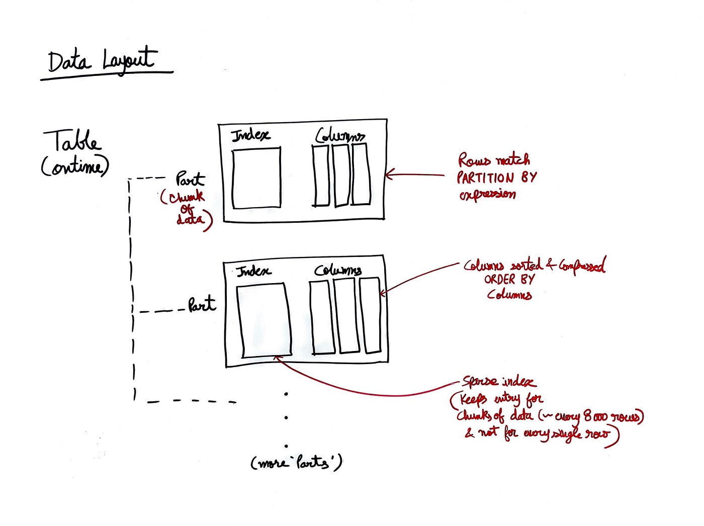
ClickHouse tables (like ontime) are stored on disk as directories called 'Parts,' with each part containing a set of files that hold the actual data and metadata.

Here’s what each component means,

Part → Chunk of data matching our PARTITION BY expression. So, for example, in our case each part could represent a specific month of data. If you don’t define PARTITION BY, ClickHouse will automatically create parts based on data insertion, without any specific logical grouping like time or categories.

Sparse Index → Stores references to data at intervals, rather than indexing every single row. In our case, this could mean indexing by month, so it knows where the entries for a specific month start, but not the exact location of every entry within that month.

Compressed Columns Data → The data is compressed using the LZ4 compression method and stored in sorted order based on the ORDER BY expression.

Let’s take a closer look at the detailed storage layout within a single part.

Inside the directory for our ontime table, /var/lib/clickhouse/data/airline/ontime, we'll find subdirectories called 'parts', each representing a chunk of data. Within each part, we'll typically see files such as primary.idx, .mrk, and .bin

Below is a pictorial representation of how it looks:

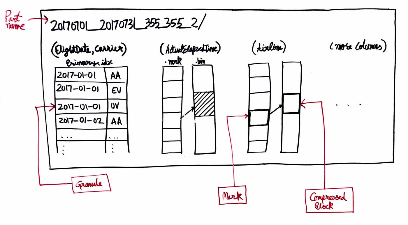
So, what are those files? What is a Granule, a Mark?

When we insert data into our ontime table, ClickHouse organizes the data into parts (we know that), based on our PARTITION BY expression. For example, we might have parts that represent each month of flight data. However, within each part, ClickHouse breaks the data down further into smaller pieces called granules. Unlike partitions, we don’t define how granules are created—ClickHouse does it automatically.

How are granules made?

• ClickHouse uses a default granule size of around 8192 rows. So, if we have a part that holds flight data for an entire month and it contains 100,000 rows, ClickHouse will break this part into smaller granules of 8192 rows each (which would give us about 12 granules).

• Granules are important because ClickHouse reads data in these manageable chunks to optimize memory usage and speed up queries.

Think of granules like chapters in a book. If you want to find something specific, you don’t want to read the whole book — you just want to jump to the right chapter. Similarly, granules let ClickHouse read only the necessary chunks of data for your query, without loading everything into memory.

So, in our ontime table, ClickHouse might create one part for January’s flight data, and inside that part, it will break the data into granules — each granule containing a fixed number of rows. When you run a query, ClickHouse will use these granules to quickly find and read only the relevant flight data, speeding up the process.

And, yes, you guessed it right — The Sparse index is the entry/index of each granules and not each entry. Sparse indexes keeps track of those granules.

So, essentially,

• Part: A chunk of data stored in a directory. Think of it as a major division in the table, often based on partitioning.

• Granules: Smaller units of data inside the part, broken down into manageable blocks.

• primary.idx: Index file used to quickly find relevant granules.

• .mrk files: Markers to find where each granule starts in the compressed data.

• .bin files: Compressed columnar data stored on disk.

Let’s see how a query would flow in ClickHouse,

1. A query is run, and ClickHouse checks the primary.idx file to find the relevant granules.

2. Using the .mrk files, it locates the starting points of the required granules in the .bin files.

3. ClickHouse then reads and decompresses only the necessary granules from the .bin files, speeding up query execution

Now, if you are like me then you may be thinking, if the primary index has the information of granules, then why can’t it also holds where each of those granules starts in the compressed data in .bin files? Like, why do we even have .mrk files? Well, here’s why,

The .mrk (mark) files contain granule-level offsets for the .bin files, which store the actual data for each column. These files mark the exact byte offsets where each granule starts in the compressed .bin files, allowing ClickHouse to quickly skip to the right position and read the necessary granule data without decompressing or scanning the whole file.

Why Can’t This Information Be Combined? Because primary.idx is focused on filtering and locating the granules based on the primary key & .mrk files are all about efficient data retrieval from the .bin files. Since .bin files store compressed column data, ClickHouse needs a way to quickly jump to the right position inside the file, and this is what .mrk files do.

If you stored the mark information in primary.idx, it would have to mix row-level offsets with key indexing. This would:

• Increase the size and complexity of primary.idx, making it slower to process.

• Make it harder to decouple key lookups from data access.

A simple analogy for understanding this is to think of it like this,

• primary.idx is like the table of contents in a book — it helps you find the chapter (granule).

• .mrk files are like page numbers — it tells you where each section of the chapter starts.

I hope it is a little clearer now. Moving on.

One more thing, the way the data is compressed in .bin is done using the LZ4 & ZSTD compression methods, which is very interesting to say the least. Unfortunately, that is not the focus of this article, i will save it for another one.

Materialized Views

Let’s Talk About them,

In the world of ClickHouse, materialized views are a special type of view that physically stores the results of a query in a table. Unlike regular views, which simply save the query definition and run it each time they are accessed, materialized views store the data produced by the query at the time the view is created or updated.

So, the process looks like this:

• Precomputed Results: Materialized views save the results of the query.

• Automatic Updates: They automatically update when the source table changes.

• Faster Queries: This allows for much faster query performance on specific use cases.

Materialized views store these precomputed query results, enhancing performance for queries that align with the materialized data. However, queries that do not match the precomputed data will run at normal speeds, directly querying the source table.

Let’s consider a scenario, where we want to analyze flight delays by month and calculate the average delay for each flight route to improve operational efficiency. Running complex queries on the original ontime table can be slow, especially with large datasets.

Here, we can create a Materialized View that precomputes the average delay per flight route by month.

CREATE MATERIALIZED VIEW avg_delay_per_route
ENGINE = SummingMergeTree()
PARTITION BY toYYYYMM(date)  -- Partition by month
ORDER BY (origin, dest)  -- Order by origin and destination
AS 
SELECT 
    origin, 
    dest, 
    toYYYYMM(date) AS month, 
    AVG(arr_delay) AS avg_delay  -- Calculate average arrival delay
FROM 
    ontime 
GROUP BY 
    origin, 
    dest, 
    month;

The Materialized View avg_delay_per_route stores the precomputed average arrival delay for each flight route (defined by the origin and destination) for every month.

Whenever new data is added to the ontime table (e.g., new flight records), the materialized view automatically updates, ensuring that the averages are current without requiring complex calculations during query time.

Here’s how we can query the view,

SELECT 
    origin, 
    dest, 
    month, 
    avg_delay 
FROM 
    avg_delay_per_route 
WHERE 
    origin = 'JFK' 
    AND dest = 'LAX' 
    AND month = 202308;  -- August 2023

Some common and practical use cases of Materialzed views are,

• Aggregation

• Automatic reads from Kaka

• Build pipelines using chained views

• Pre-computing last-point queries

• Changing primary and sorting key

Table Engines

What about Table Engines? Why So Many Table Engines in ClickHouse?

Table engines in ClickHouse are specialized storage formats that optimize how data is organized and queried. Each engine is designed for specific use cases, such as handling large volumes of data, optimizing read and write performance, or enabling real-time data processing. By selecting the appropriate table engine, users can tailor their database to meet their unique data handling and performance requirements.

Think of ClickHouse as a magical airport for your ontime data, where different table engines help you manage the flight schedules in the best way possible. Here’s how it works:

• Speedy Departures: Some engines are like express flights! They’re designed to get you results quickly, just like how you’d want to check flight delays and arrivals in a flash.

• Tailored for Different Flights: Just like not every flight needs the same kind of service, different engines cater to different types of data. If your ontime data is frequently updated with new flights, the CollapsingMergeTree engine swoops in to keep things tidy and organized.

• Prepped for Efficiency: Imagine you want to quickly check how many flights are delayed this month. The AggregatingMergeTree engine can have those numbers ready and waiting, so you don’t have to search through every flight individually.

• Flexibility at the Gate: Just like a good airport adjusts to passenger needs, ClickHouse allows you to choose the right engine for your specific ontime data needs. Whether you’re tracking thousands of flights or just a few busy routes, there’s an engine that fits perfectly!

So, with these engines ready to take off, ClickHouse ensures your ontime data is always flying smoothly!

Below are some common table engines:

• MergeTree: The default engine designed for general-purpose OLAP workloads. It’s great for handling large datasets with efficient reading and writing operations.

• AggregatingMergeTree: This engine is optimized for aggregation queries. It precomputes aggregates, which makes querying summary data incredibly fast.

• CollapsingMergeTree: Ideal for scenarios with frequent updates, this engine helps keep data consistent by collapsing rows that share the same primary key. Think of it as a way to merge similar entries.

• ReplacingMergeTree: Similar to the CollapsingMergeTree, but instead of collapsing, it replaces older rows with newer ones based on a specified version column. This is perfect for ensuring that you always have the latest state of your records.

• DistributedMergeTree: This engine is designed for handling distributed data across multiple nodes. It allows you to run queries on data that’s spread across different servers, providing scalability and performance.

• ReplicatedMergeTree: This engine adds a layer of high availability by automatically replicating data across nodes. If one node fails, the data is still accessible from another, ensuring that your applications remain online.

Scaling

If you’re still with me at this point, you’re in for a treat! Let’s dive into some exciting new information. How can we scale our ClickHouse database?

ClickHouse knows how to make the most of your hardware, pushing it to its limits and using every bit of power your machine has to offer. Generally, it’s a good idea to scale up (vertically) before considering scaling out (horizontally) — that way, you can enjoy better performance until the costs of scaling up starts to climb too high.

Scaling out — often referred to as sharding — should be considered only when you anticipate a significant increase in data volume or processing speed that may soon exceed the capacity of a single server.

You might reach the limits of a single server’s capacity if:

• The amount of data becomes too large.

• The request rate grows beyond manageable levels.

• Data processing speed slows down significantly.

When you add an additional host to your ClickHouse cluster, you can split or shard the data of a table into two tables. This effectively doubles the capacity of your ClickHouse setup, allowing for increased data volume and enhanced processing speed.

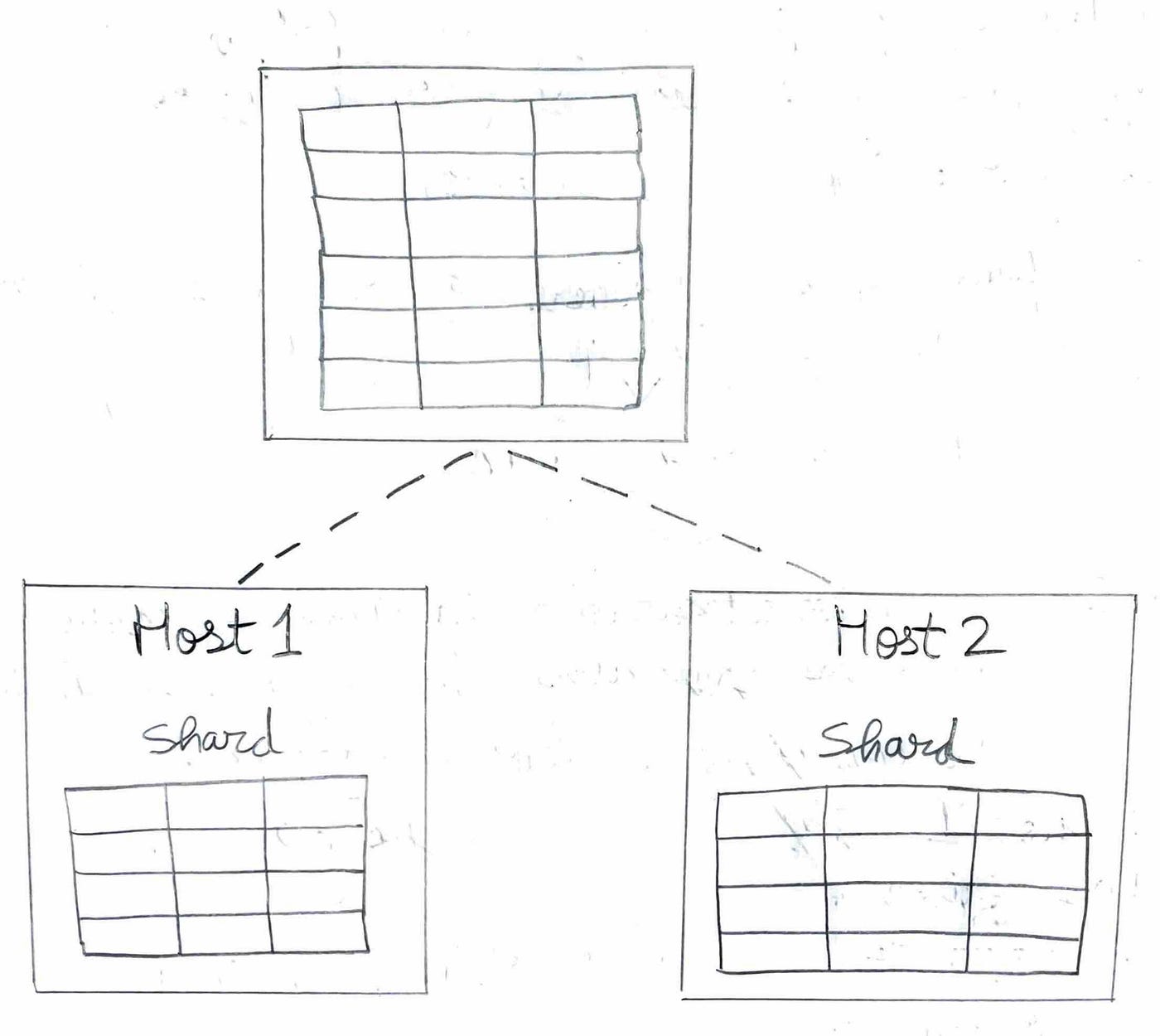
The ClickHouse approach to sharding is very low-level due to its shared-nothing architecture. For example, there is no coordination between the cluster hosts; the two tables on host 1 and host 2 are completely independent of each other.

For convenience, a Distributed table can be created. A Distributed table doesn’t store any data by itself but provides a single table interface for combined access to remote tables located on different hosts. A Distributed table can be created on one or multiple hosts.

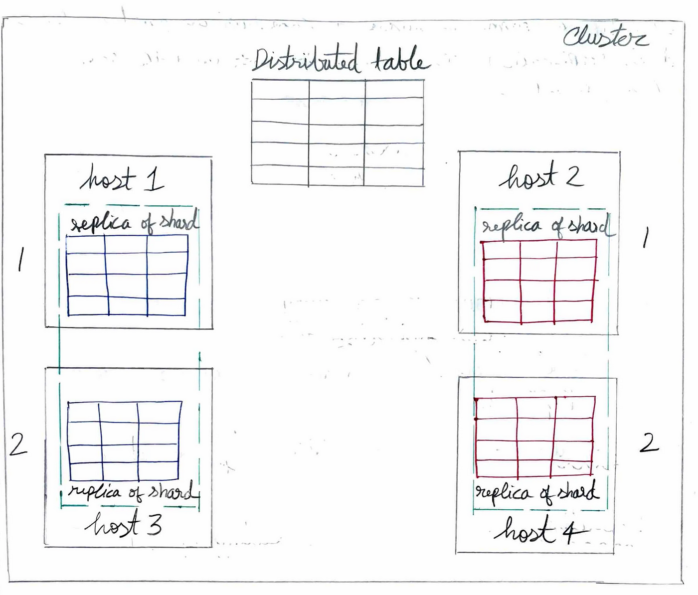
• Two or more hosts can be added to the cluster to replicate table data. Now, each shard has multiple copies of the data, and new data can be written to any replica of a shard, with the other replicas automatically syncing these changes.

• Replication ensures data integrity and provides automatic failover in ClickHouse.

For replication, an additional component is required: ClickHouse Keeper.

ClickHouse Keeper acts as a coordination system for data replication, notifying the replicas of a shard about state changes. It serves as a consensus system, ensuring that all replicas of a shard execute the same operations in the same order.

Note: ClickHouse Keeper only stores metadata for ClickHouse. Additionally, sharding and replication are completely independent of each other.

Replication: Ensures data integrity and automatic failover.
Sharding: Enables horizontal scaling of the cluster.

If sharding is not needed, we can simply use replication to make our data highly available.

Well, that concludes a very surface-level introduction to various concepts of ClickHouse. I hope it gave you some insight into ClickHouse and got you at least a little excited about it! If you learned something new or just want to share your thoughts, let me know in the comments!

Later 👋  

This article is inspired by and incorporates information from the following sources:

• https://www.youtube.com/watch?v=fGG9dApIhDU&list=LL&index=22&t=179s&ab_channel=CMUDatabaseGroup

• https://www.youtube.com/watch?v=vBjCJtw_Ei0&ab_channel=ClickHouse